Taught by Professor Brenda Davison
Convergence
Newton's Method
This is an iterative method to solve for roots of a polynomial function.
the idea is \(x_{n+1} = x_n-f(n)/f'(n)\). Every iteration we are approaching the root.
Note, this method depends on a good initial point. The derivative have to be fairly steep , and not zero.
To know when to stop, we need to check to see what criteria the questions asks for. usually its relative tolerance, and the format is \(|p_4-p_3| < 10^{-x} \) where \(10^{-x}\) is a stopping criteria.
converges quadtratically, has order of 2,
Secant Method
When we can't easily get the derivative of a function, we can use the secant method. The downside is secant method is slower, and also it needs two initial values
Bisection Method
The idea is to bracket the root with our guess.
we have to get a and b, such that f(a) * f(b) < 0 , so opposite signs.
then we find \(c = (a+b)/2\) , and we check if \(f(c)==0\) otherwise we set a to c, or b to c depending on the sign.
and repeat iteration
Bisection is guranteed to converge, per the intermediate value theorem.
Interpolation
Cubic Spline
Method for finding out the natural cubic spline
- \(S^2_0(0) == S^2_1(0) == 0\)
- \(S_0(0) = f(0) S_1(1)= f(1) , S^1_0(0) = S^0_0(0) , S^2_0(0) = S^2_1(0) \) this is saying at the given data point, it must match (this is the main idea of interpolation)
Computing Assignments Takeaways
CA 1. Effects of calculating irrational numbers
When we repeately calculate irrational number, the number gets truncated at some point. accumulation of rounding error occurs. Most computers follow IEEE standards for floating points, (in 64 bits floating points, the mantissa can only hold 52 bits).
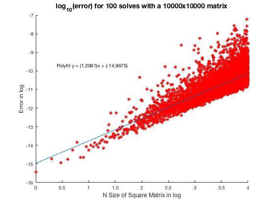
CA 2. Gaussian Elmination on a large random matrix
The larger the square matrix in the matrix operation. The more prone to rounding errors. The error grows linearly with respect to log N.

CA 3. Ill-conditioned linear systems
We investigated how ill-condition linear systems behave when factorized. An ill condition system has high norm and condition number, and higher than 1 is no good. the idea is that in a well condition system A * A' should be 1.
We also compared factorization techniques vs hilbert matrices. We saw that LU factorization had the highest 2-Norm error, the QR factorization had the lowest error, and the matlab's backslash is between the two.
However the running time of QR was the slowest, follow by Matlab backslash, then LU factorization.
CA 4. Finding zeros of Bessel functions
We wrote our own bisection methods to do zero-finding (root finding) for a bessel function. Bisection methods use two points of opposite sign, and repeatedly close in on the root that is in the middle. We confirmed that bisection is a robust, and accurate method for root finding.
CA 5. Polynomial interpolation and node distribution
We investigated the relationship between the spacing of points and the error in interpolation. Using Equidistance points in polynomial interpolation causes Runges phenomenon, which is when the polynomial oscillates wildly outside of the boundary points.
It is better to use chebyshev nodes, which are nodes that are more distributed towards the boundary of the interval.
CA 6. Finite Difference Method (for numerical differentiation)
We compared the forward difference, backward difference, and central difference method for finding the derivative of a function.
We found that forward difference and backward difference are considered \(O(h)\) and central difference \(O(h^2)\). So central difference is more accurate.
CA 7. Trapezoidal rule
We used trapezoidal rule to estimate the integral of a function. We found that trapezoidal rule is really accurate for some functions, such as cosine, and sine in a periodic range. This is due to way trapezoidal rule is calculated, and the periodic wave 'cancels' each other out. In general, as the number of data points increase, the trapezoidal rule gets more and more accurate.
Trapezoidal rules have a rate of convergence of -2, because the slope is given by \(log(Error)/log(N) = -2 \)
CA 8. Numerical Solution of Kepler’s problem (Initial Value Problem)
We compared Euler method in solving the Kepler planetary motion. We found that euler method is not accurate for this problem due to truncation error. Instead, we should use the sympletic euler method instead because they are semi implicit, whicih uses a newton's iteration to find the solution at the next step.